
Welcome to the NanoTube!
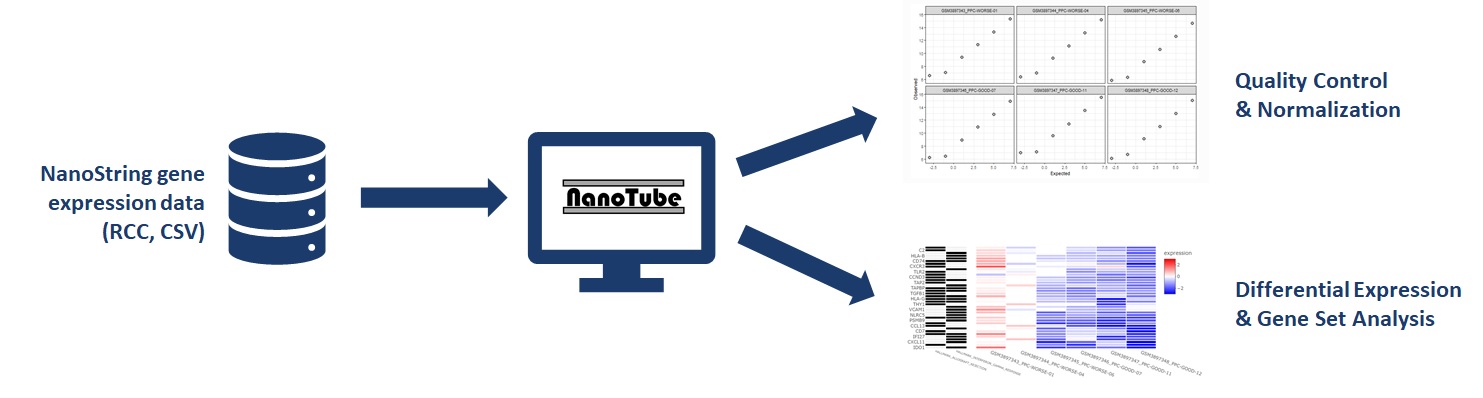
NanoTube performs data processing, quality control, normalization and analysis on NanoString gene expression data.
Click on the Setup tab to get started.The downloadable version of this R-Shiny application can be found on GitHub, along with example data sets.
Check out the NanoTube package on Bioconductor!This R package provides additional normalization and analysis options for NanoString nCounter data.
Basic Features
Data Processing
nCounter data are input as raw RCC files or CSV files (which possibly came from the RCC Collector tool). An additional sample information table is then loaded to allow comparisons between groups.
Normalization
This application performs manufacturer-recommended normalization steps, including positive and housekeeping normalization, as well as the removal of target genes found to have expression levels below 'background' (estimated from the negative control gene expression). Alternatively, the RUVg normalization method has been demonstrated to perform well using housekeeping genes.
Analysis
Differential expression analysis is conducted using Limma (the NanoTube R library also allows DE analysis using NanoStringDiff). Gene set analysis is conducted from the ranked DE results, using the fgsea package.
Visualization
This application provides basic visualizations for quality control, including observed/expected plots for positive control reporters, boxplots to assess normalization performance, and PCA plots. Volcano plots and heatmaps are provided to interactively explore the results of differential expression and gene set analysis.
Citation
If you use the NanoTube in your work, please cite our paper:
Class CA, Lukan CJ, Bristow CA, Do K-A (2023). Easy NanoString nCounter data analysis with the Nanotube. Bioinformatics 39(1). DOI: 10.1093/bioinformatics/btac762
License
The NanoTube and its Shiny app are provided with the GNU General Public License (GPL-3), and without warranty.
GPL-3 License for NanoTube
Data Entry
Advanced Options
Normalization Options
Gene Set Analysis Options
Observed-Expected Plots
Sample Size Factors (Positive Controls)
Endogenous Targets vs. Negative Controls
Target Statistics
Sample Statistics
Negative Target Counts
Housekeeping Assessment
Raw Data
Normalized Data
Sample Size Factors (Housekeeping Genes)
Normalization Assessment
Raw Data
Normalized Data
PCA
Volcano Plot
Summary
Full Results
GSEA Visualization Options
Setup
NanoString data
Your NanoString data should be loaded as a ZIP folder containing one RCC file per sample, or a CSV or TXT file containing expression data for all samples.
Sample info table
This field requires a CSV file containing sample information. This Shiny app conducts group-vs.-group comparisons, so one column must include the group identifier for each sample (for example, Treated or Control). Sample names should be in the first column. If the RCC filenames are used as sample names, they will be merged so that they match. Otherwise, the RCC files and sample table will be merged in the order they're supplied. The merge can be checked prior to analysis using "Check Samples", to make sure they match.
Advanced: Design Matrix Input
Check this box only if you input a Design Matrix as described here.
For more complex experimental designs (for example, involving multiple factors or
numeric factors, you can load a Model Matrix (or Design Matrix) in this step.
This should be input as a csv or txt file (similar to the sample info table),
where each row is a sample and each column is a factor. This can be generated
manually or using R, with the model.matrix() function. For proper functioning in this web app, the first column should be
the Intercept term (equal to 1 for all samples), and other columns should be 0/1 for group variables (not including
control group) or numeric for numeric variables. An example model matrix is provided in the data folder of the
Shiny-NanoTube github repository.
Group Column
After loading the sample info table, a dropdown box will appear, containing the columns from that table (such as the "Treatment" column). Select the column containing the group information for differential expression analysis.
If the user input a design matrix instead, the "Group Column" and "Base Group" options are not shown.
Base Group
This is the group that all other groups will be compared against (i.e. the denominator in your Fold Change). For example, if your data contain groups "A", "B", and "C", and you select "C" as the base group, NanoTube will conduct analyses and calculate fold changes for A vs. C and B vs. C.
Gene Set Database
Required only for Gene Set Analysis feature. Gene set database (gmt format, such as those found at MSigDB) can be loaded here. An rds file could also be loaded, containing the gene set database in list form (each member of the list is a vector of genes from one gene set). Alternatively, the REACTOME database can automattically be used without inputting any database file, by selecting the checkbox below the Gene set database input.
Reference: Gillespie M et al. The reactome pathway knowledgebase 2022, Nucleic Acids Research. 2021; gkab1028, https://doi.org/10.1093/nar/gkab1028
Advanced Options
Normalization Method
The Shiny app allows normalization using either the standard "nSolver" method, which conducts scaling normalization using positive control and housekeeping genes; or with the "RUVg" method (Risso et al., 2014), which Removes Unwanted Variation based on housekeeping genes.
Housekeeping Genes
NanoTube will automatically identify housekeeping genes for normalization by selecting those marked as "Housekeeping" in the CodeClass. Alternatively, these can be manually specified with this option, by inputting a comma-separated list of genes to be used as housekeeping genes.
Negative Control Threshold
This step can be applied with any normalization method. The NanoTube app performs a two-sample, one-sided t test for each gene: this test compares the expression of that gene across all samples vs. the expression of all negative control genes across all samples. The p-value of this test is for the null hypothesis that the endogenous gene does not have expression above the negative control genes. In this field, you can specify the signifance level required to keep a gene for analysis. A lower value is a more stringent threshold: genes with a p-value above this level will be removed, and not included in differential expression or gene set analysis. To skip this step, this value can be set to 2.
Number of Unwanted Factors
User can specify the number of unwanted factors to remove from the data (for RUV normalization methods only). 1 is usually a good first guess, but it may need to be increased if variation based on batch/unwanted effects remains.
Number of Singular Values to drop
The number of signular values to drop when estimating unwanted variation factors (RUVg normalization only). 0 is a good first guess for this one, but it could be set to 1 if the first singular value captures the effect of interest, for example. This number must be less than the number of unwanted factors.
Minimum Gene Set Size
In this field, you can set the number of genes required for an individual gene set (from a loaded gmt file) to be included in analysis. For example, if this value is set to 5 (default), only gene sets with at least 5 genes present in your data set will be included in gene set analysis.
Quality Control
Positive Controls
The NanoTube web app identifies positive control, negative control, and housekeeping genes prior to analysis, mainly based on each gene's CodeClass in the input data. If "nSolver" normalization was selected, positive control normalization is performed by scaling all genes by the Scale Factor for each sample, calculated using the geometric mean of the positive control genes. This scaling is not conducted for "RUVg" normalization, but the scale factors are provided for QC purposes. Scale factors outside of the range 0.3-3 indicate high variance between samples and potential problems in the data, and these should be checked before proceeding.
A scatter plot of Observed vs. Expected expression of positive control genes is also provided for each sample, with the R-squared values provided in the table. "Expected" expression is identified from the positive control gene names. Low R-squared values potentially indicate issues in detection of the positive control genes.
Negative Controls
The Endogenous Targets vs. Negative Controls table shows how many of the endogenous genes "passed" the comparison with negative control gene expression (defined in the Setup section). Genes that did not pass are removed, and not included in the analyses. The comparison statistics of each gene against the negative controls are presented in the Target Statistics table.
A table showing Sample Statistics for the detection of negative control genes within each sample is also provided, including the average, maximum, and standard deviation of negative control gene detection. In addition, a threshold "Background" level is provided, and calculated using negative control gene expression as cutoff = mean + 2*sd. The number (and percentage) of endogenous genes with average expression below that level is presented for each sample. Samples with a high percentage of genes detected below background level may present a quality concern.
Finally, a scatter chart of the detected counts of each negative control in each sample is also provided.
Housekeeping
As with positive control genes, a scale factor is calculated using the geometric mean of the housekeeping genes for each sample, and this is used to normalize the endogenous genes ("nSolver" method only). Housekeeping genes are automatically detected from RCC files, or they can be manually entered in the Advanced Options on the "Job Setup" tab. This scaling is not conducted for "RUVg" normalization, but the scale factors are provided for QC purposes. Scale factors outside the range of 0.3-3 indicate high variance between samples, and should be checked before proceeding.
Box and jitter plots of Relative Log Expression (RLE) are also provided for each housekeeping gene across samples, both before and after normalization. Housekeeping genes exhibiting particularly high variance after normalization indicate that these genes are not in accordance with other housekeeping genes and may need to be removed. This can be done manually in the Shiny app: go back to "Setup" screen, and input the desired Housekeeping genes in the "Advanced Options" menu.
Normalization Assessment
Boxplots of endogenous gene expression before and after normalization are also provided in this tab. These can be plotted using the log2(Expression) values, or using the Relative Log Expression (RLE) method described by LC Gandolfo and TP Speed (PLOS One, 2018).
Analysis
PCA
A simple Principal Components Analysis is performed using the 'prcomp' function, and a scatterplot of the first two principal components is drawn here. Samples are represented as points, colored by their Group membership, and specific sample names can be identified by hovering over the points.
Volcano Plot
A volcano plot of the selected group vs. the base group is drawn here. Alternatively, if DE analysis was conducted using a design matrix, you can select a design factor for the volcano plot. Fold change is calculated as FC = (Selected Group / Base Group), so genes on the right of the plot have higher expression in the Selected Group. A log2(FC) and nominal p-value cutoff can be defined in the boxes, to draw vertical and horizontal lines (respectively) on the plot. Target names (such as gene symbols) can be identified by hovering over the points.
Differential Expression
For each analysis of Group vs. Base Group (indicated in parentheses), a table containing the following four columns is provided:
Log2FC: The log2 fold change of each gene, calculated as log2(Group / Base Group). Genes with positive log2FC have higher expression in "Group", while those with negative log2FC have higher expression in "Base Group".
t: The comparison statistic calculated by 'limma'.
p-val: The nominal p-value calculated by 'limma'.
q-val: The p-value adjusted for multiple testing, using the Benjamini-Hochberg procedure.
Gene Set Analysis
Gene set enrichment analysis is conducted using the 'fgsea' preranked package, resulting in a table of statistics and a heatmap of gene expression within specified gene sets.
Options
Comparison: The group that will be compared against the base group.
Clustering Threshold: Gene sets containing similar genes are clustered together to ease the interpretation of results. The overlap between two gene sets is calculated as the Jaccard index, the genes overlapping between the sets divided by the union (total genes) of the sets. Sets with an overlap greater than the clustering threshold will be "clustered" together. Moving this slider to the left will result in more gene sets being clustered together.
q-value Threshold: Only gene sets with a q-value (p-value adjusted for multiple testing) below the threshold will be included in the table or heatmap. Use a threshold of 1 to include all gene sets.
Cluster to plot: The gene set "cluster" to plot in a heatmap. The assigned cluster for each gene set can be found in the results table; a cluster may contain one or more gene sets.
Result Table
This table contains the standard gene set analysis statistics for each gene set, based on the options set by the user. "p.adj" is equivalent to a "q-value", and the NES provides the normalized enrichment score, or the direction of the enrichment. Gene sets that are more highly expressed in the "Group" will have a positive NES, while those highly expressed in "Base Group" will have a negative NES.
Gene sets are clustered using the Jaccard index (as defined above), and the gene set with the lowest p-value within each cluster is defined as the "most enriched" gene set of the cluster ("Cluster.Max"). The developers generally recommend that the user focus on the gene set within each cluster with the lowest p-value, as this one may be responsible for the detected enrichment of the other gene sets. However, this recommendation is not absolute, as multiple similar pathways may be providing unique contributions.
Heatmap
A leading edge heatmap for a "Cluster" of gene sets can be plotted by specifying which cluster in the options. Cells are colored based on the log2(expression) for each gene in each sample, centered on the median of the "Base Group". If there are more than one gene set in the cluster, gene set membership information is also provided in the heatmap.